pls i want help on my project development of number system with their needs

On Numbers

Prehistoric Origins of Numbers

Numbers are abstract ideas used in designating quantities, as in counting or measuring. The origin of numbers is prehistoric, in the Paleolithic period. Early physical evidence of the use of numbers by humans dates from 30,000 B.C. and takes the form of a wolf bone found in eastern Europe, with a series of notches carved in it, which seem to represent a tally of some kind. There was a need among our ancestral hunter-gatherers for a way of distinguishing between one and many, be it days, offspring, prey, or feared predators. The use of numbers may predate Homo sapiens.

Tallying and Counting

Tallying is likely to have predated counting and the use of words to denote specific quantities. A tally system might have been used to keep track of the days in a lunar month. A notch may be carved in a stick for each night after a full moon, until the next full moon, and the notches may be marked off to predict the beginning of subsequent lunar months. This could be done without enumerating the nights in a month.

Every known human language has a word for one, a word for two, and a word for many. Among some prehistoric peoples, the one, two, many system may have been extended to allow the representation of groups of three or four objects by repeating the representations for one or two. Three would be two-one, and four would be two-two. This need not have involved counting, or the concept of an increasing series of numbers, but the need to track particular occurrences.

Counting may have evolved nearly as early as speech. There were compelling evolutionary pressures to be able to communicate a distinction, not necessarily a precise distinction, between the sudden appearance of two, six, and eighteen gazelles. The pressure may have been greater if, instead of gazelles, hostile tribesmen were observed.

Our ancestors may originally have had a word for three people and another for three axes. An abstract idea of number may have occurred to an intellectually gifted ancestor who developed the concept of “threeness,” perceiving that a group of three deer and three spears had something in common. Communicating this concept to others would have led to the invention of a word for “three.”

In early forms of speech the number five was often expressed by the word for hand, and ten by two hands. Sometimes twenty was expressed as “all the fingers and toes.” Six was spoken as “one of the other hand,” and so forth. A number indicating a quantity, for example, the number of people in a family, is called a cardinal number.

Ordinal Numbers

Ordinal numbers indicate position in a sequence, for example, first, second, third. The development of ordinal numbers may have originated from using fingers and toes to count on. If done in the same order, say starting with the little finger of the left hand and proceeding towards the left thumb, then the same finger will always be used to represent a particular quantity. This associates the position of items in a sequence with the order in which fingers are arranged. This association is not present if pebbles are used to perform a tally. Any pebble in a pile could be the fourth one, but only the fourth finger would indicate the fourth item in a sequence.

Pictorial Representations

Earlier members of the human family, such as Homo erectus, did not leave evidence of an ability to draw or paint. Drawings and paintings in cave walls first appeared about 30,000 B.C., and are associated with Homo sapiens, anatomically modern humans. The drawings suggest that prehistoric peoples had the ability to hold in the mind a vision of something seen in the past, and of recreating the image in the form of a painting or drawing. Some of the cave walls where paintings of horses, bison and deer have been found, also show symbols, some of which may be tallies.

Neolithic Ideograms and Tokens

There is archaeological evidence of people gathering and processing seeds as early as 21,000 B.C., and of organized farming and domestication of animals in the Mesolithic period, around 10,000 B.C. The development of tiny flint tools, flaked in two directions and set in bone or wood, allowed making precise markings and facilitated tallying.

The need to keep track of fields, crops, and herds was a major impetus for the development of ideograms, mnemonic symbols, and tokens in the Neolithic period, around 7000 B.C. Widespread dairy farming was made possible at about 6000 B.C. by a mutation in European and some African populations that allowed the production of lactase, and the consumption of milk, into adulthood. Agriculture and animal husbandry led to larger and more permanent groupings of people and to settlements.

Settlements evolved into villages, and some Neolithic villages evolved into largely self-supporting towns with populations of several thousand. Early forms of farm management, commerce, the reckoning of time, and genealogy led to the development and use of ordered lists.

Since planting and harvesting are best carried out in appropriate seasonal conditions, agriculture provided an incentive for the study of seasonal changes in climate and for the accurate reckoning of time. Words for month and year have prehistoric origins in ancient languages. The adoption of the month and year as terms for discrete numbers of days implies the ability to reckon, through tallies or counts, quantities of days for the lunar month and for the solar year.

One use of lists was in systems of tokens used to represent commodities. The tokens represented specific objects. Different types of goods were represented by different tokens. Quantities were represented by repetition. Five rectangular pebbles in a particular tray could represent five bags of grain from a specific individual. A jar of oil could be represented by a little figure of a jar.

At some point, it occurred to someone to create a token to represent a number of objects, to make it more expedient to record larger quantities. For example, a rectangular pebble with an inscribed mark could be used to represent twelve bags of grain.

Pictographs

By 4000 B.C., the development of copper tools facilitated the working of wood and stone and the making of precise inscriptions in a variety of materials. With increasing population and degree of division of labor, the earliest cities appeared about 3700 B.C. At about that time, two more-efficient means of recording information were developed: ink markings on papyrus paper and impressions on clay tablets. The information was recorded in the form of pictographs, in some cases representations of the earlier tokens.

Over time, pictorial representations were simplified and became more abstract. Symbols, possibly primitive words, have been found etched in Indus Valley Harappan pottery dating from about 3500 B.C.

Symbolic representations of words and numbers took various forms and were developed in locations ranging from Egypt to Mesopotamia and the Indus Valley.

The several original representations differed in breadth, form and concept. In diverse locations, ancient bookkeepers, builders, priests and tax collectors had needs to record information, for their own purposes. Different methods for representing words and numbers were developed, not only in different regions, but for different applications within the same location. Over time, consistent representations were adopted over broad areas.

Numerals

Egyptian hieroglyphs and Mesopotamian scripts were developed in the Bronze Age, by 3200 B.C. These were standardized methods for writing words and numbers.

At some point, the representation of the quantity of an object was separated from the symbol for the object. A symbol used to represent a number is called a numeral.

The Egyptian Number System

The Egyptians had three systems of writing: hieroglyphic, hieratic, and demotic. Hieroglyphs were the sacred writing used for formal inscriptions, usually on stone. They were written from right to left or left to right, starting from the direction the figures face. Upper figures were written before lower figures. Numbers were used sparingly, typically to date events and to identify rulers.

Hieratic writing was a simplified version of hieroglyphs used by priests and scribes for common records mostly written on papyrus. Demotic writing was a further simplified method developed from hieratic writing. It was used in everyday life, often to record numbers.

Egyptian numbers were decimal and were represented by pictographs. The numbers one to nine were written as combinations of vertical strokes. Special symbols were used for the numbers ten, one hundred, one thousand, etc. If appearing together, the Egyptian numerals shown represent the number one thousand one hundred and eleven.

Rational Numbers

The use of fractions originated with the Egyptians. Fractions lead to the concept of rational numbers, which are different from the natural numbers one, two, three, four, etc. A rational number (fraction) expresses a ratio of two integer quantities, for example, three eighths is the number of eighths of a bar of gold taken in payment, and eight is the total number of eighths that make up the whole bar. Each rational number can be expressed in many ways. One third, two sixths, and four twelfths, all have the same value.

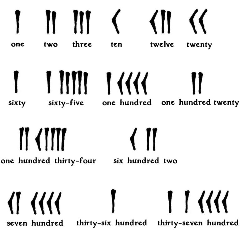
The Sumerian Number System

The Sumerians were originally peoples from the Caucasus that moved into southern Mesopotamia about 4000 B.C. They devised a system of writing based on symbols incised in clay with a stylus. Accountants developed number systems based on circles and cones impressed in clay. The cone was the unit symbol, and the circle signified a number of units, typically six or ten. The value of a symbol depended on its place in a series of symbols. Reading from the right, values increased by a factor of ten or sixty. Initially, different conventions were used to enumerate different kinds of objects, but standardization occurred over time. The original pictograms were, over centuries, further developed into a simplified system of writing using ideograms called cuneiform.

By around 2200 B.C., the Sumerians were using a place-value sexagecimal number system that had only two numerals. A vertical stroke was the unit symbol, and a wedge was the ten numeral.

The rightmost position represented the numbers one through fifty-nine. One vertical stroke represented the number one, two strokes represented the number two, nine strokes the number nine. One wedge represented the number ten, two wedges the number twenty. A unit numeral (the vertical stroke) in the second position had a value of sixty (60¹). A space was used to separate numerals in the first (rightmost) position from those in the second position. The vertical stroke symbol in the third position had a value of thirty-six hundred (60²).

When representing the number sixty, the place to the right had no value, so that the number sixty was represented the same way as the number one. This ambiguity was resolved by referring to the context in which the numbers appeared.

We still use a base sixty system for seconds in a minute, and for minutes in an hour. Counting boards, similar in concept to the abacus, were used to aid in computations. These boards were shaped like a checkerboard, with rows and columns used to represent numbers.

Babylonian Numbers

About 2000 B.C., the Babylonian civilization replaced the Sumerian and Akkadian nations in Mesopotamia. The Babylonians used a positional base sixty number system derived from the Sumerian system.

Babylonian numbers were written from right to left and used two basic cuneiform numerals: the unit symbol and the ten symbol. As in the Sumerian system, other numerals were formed by combining the two symbols. The rightmost place was for values from one to fifty-nine, the next place to the left was for multiples of sixty through 3540, etc.

When representing a number that was a multiple of sixty, the place to the right had no value, so that the number sixty was represented the same way as the number one, and one hundred and twenty the same way as two. The Babylonians got around this ambiguity by relying on context to determine the trailing places with no value, and by leaving an empty space where a place with no value occurred elsewhere. This was not an ideal situation, and around 400 B.C. scribes started to use an additional symbol, a positional null, or zero, to denote an empty place.

The Greek Number Systems

By around 900 B.C., the ancient Greeks were using the Herodian number system. This system was decimal like the Egyptian system and used the initial Greek letters of the number words to represent the numbers. The Greek alphabet was itself derived from the Phoenician syllabary.

 Ι one   Γ five   Δ ten   Η one hundred   Χ one thousand

Small versions of the numerals for ten, one hundred or one thousand were appended to the symbol for five to create numerals for the numbers fifty, five hundred, and five thousand.

Greek scholars made significant advances in mathematics. They devised mathematical equations and used geometry for theoretical and practical purposes. The ancient Greeks applied logic to develop theorems and mathematical proofs. The combination of logic and numerical series led Zeno of Elea to formulate, around 450 B.C., his paradox of the negation of motion. “To move from one place to another, you must first cover half the distance. Once there, you must cover half the remaining distance. Then, you must move across half the remaining distance. You must then cover half the remaining distance, and so on, forever. The consequence is that you can never get from one place to another. In fact, you cannot move.”

The Greek Herodian number system was replaced by the Ionian system by about 100 B.C. The Ionian system was more advanced but required the use of more than twenty-seven symbols. The Ionian numerals were based on the twenty-four letters of the Greek alphabet plus the special characters digamma, kappa, and sampi. In the Greek Ionian system, fractions were expressed by bars over the numerator and diacritical marks after the denominator.

 α one   β two   γ three   δ four   ε five   ι ten 

 ια eleven   ιβ twelve   κ twenty   λ thirty   μ forty   ν fifty 

 να fifty-one   ρ one hundred   σ two hundred   φ five hundred 

During Alexander’s Macedonian expansion to the East, the Greeks became aware of the Babylonian use of the positional zero, but few used this concept, since the Greek number system was not positional. The zero raised unsettling philosophical questions and contradicted the teachings of Aristotle.

The Golden Ratio

When the Greek sculptor Phidias and the architects Iktinos and Kallikrates designed the temple of Athena Parthenos in Athens, around 447 B.C., they made use of a proportion now called the Golden Ratio. This proportion was used earlier by the Egyptians in the construction of the pyramids and occurs in the physical universe in various ways. The Golden Ratio is a number defined as the proportion of a whole line segment Alpha to a large segment of the line, Beta, which has the same value as the proportion of the large segment, Beta, to the small segment, Gamma. The proportion is satisfied when Alpha = Beta + Gamma, and Alpha/Beta = Beta/Gamma. The value of the Golden Ratio, phi, is 1.618...

Irrational Numbers

Numbers that cannot be expressed as ratios of integers are called irrational numbers. Hippasus of Metapontum, a Greek scholar, discovered the existence of irrational numbers around 500 B.C. Specifically, he discovered that the square root of two is irrational. Around 380 B.C., Eudoxus of Cnidus provided a rigorous proof of the existence of irrational numbers. The work of Eudoxus allowed the consideration of continuous quantities and not just natural numbers and rational numbers.

Roman Numbers

The ancient Romans used a number system in which certain letters of the Latin alphabet are given numeral values. Their number system was developed by about 600 B.C. from an earlier Etruscan number system that used special symbols. The Roman number system was, like the Greek and Egyptian systems, a decimal system. Latin letters were used to represent numerals.

For large numbers a bar was placed above the base numeral to indicate multiples of one thousand.

I	II	III	IV or IIII	V
one	two	three	four	five
VI	VII	VIII	IX or VIIII	X
six	seven	eight	nine	ten
XI	XX	XXX	L	LXX
eleven	twenty	thirty	fifty	seventy
C	CC	CCCXI	D	DCC
one hundred	two hundred	three hundred eleven	five hundred	seven hundred
				__
CMXXI	M	MMVII	MMM	IX
nine hundred twenty one	one thousand	two thousand seven	three thousand	nine thousand

Roman numbers are additive, as in: three - III,  twelve - XII,  six hundred thirty-three - DCXXXIII. 
Or subtractive, as in: four - IV,  ninety - XC,  nine hundred - CM.

The Romans did not have standardized numerical representations for fractions. They represented fractions by writing them out in words, often in terms of the uncia, which was one twelfth. For example, one sixth would be written as two unciae. Following the establishment of the Roman Empire in 27 B.C., Roman numbers were adopted throughout Europe, North Africa and the Middle East. They are still used for certain applications, such as publication dates, numbered lists, and clock faces.

Chinese Numbers

The Chinese used several number systems, beginning about 1200 B.C., during the Shang Dynasty. By 300 B.C., during the Zhou Dynasty, the Chinese had developed a rod number system derived from wooden sticks used on counting boards.

Numerals from one to five were represented by an increasing number of parallel vertical strokes or rods. The symbol for six was formed by adding a horizontal stroke above one vertical stroke. Six through nine were formed by adding additional vertical strokes below the horizontal rod. A stand-alone horizontal rod was the symbol for ten. Two horizontal rods represented twenty, three thirty.

Chinese numbers used a base ten positional system. Numbers were represented in a row, with one through nine to the right, tens next, then hundreds, thousands, and so on. Blank columns were represented by a space. Hundreds were represented the same way as the units, thousands the same way as the tens, and so on, alternating.

By 50 A.D., some Chinese mathematicians used negative numbers in solving systems of simultaneous equations. Red rods were used to denote positive coefficients, black to denote negative ones. At the time, the use of negative numbers was limited to mathematical theory, since no practical use had been found for them.

The Mayan Number System

The Mayan number system was a vigesimal (base twenty) system, first adopted around 300 B.C. By 1492, when the Spanish discovered America, the Mayan civilization had mostly collapsed. Many Maya scripts that existed then were subsequently lost or were destroyed by Spanish priests worried about bloodthirsty Mayan religious rituals. The last Maya kingdom, Tayasal, fell in 1697. Persistent study of surviving materials, such as Bishop de Landa’s codex, and the discovery of new inscriptions, has allowed the reconstruction of a number system that was developed independently and yet has striking similarities to other number systems.

The Mayan system of numerals at first used only two basic symbols, a dot and a bar. The numbers one through four were represented by a corresponding number of dots. Five was represented by a horizontal bar. The other numbers were represented by combinations of dots and bars. Six was a dot above a bar. Ten was two horizontal bars, fifteen was three bars. The symbol for twenty was a dot, the same as the symbol for one.

At some point before 400 A.D., the Mayans adopted a symbol to represent a null or zero value; this symbol was similar to a conch shell and was used to clarify the position of the multiples of twenty. Twenty was thereafter represented by a dot above a shell. The shell symbol indicated a positional zero.

In addition to the dot and bar system, Mayan numbers were expressed for commemorative purposes in terms of face glyphs. Each numeral through nineteen was associated with a unique face glyph.

The system used for dates in Mayan calendars was a variation of a pure base twenty system, in that the third position was eighteen rather than twenty, to make it easier to represent the number 360 (twenty times eighteen).

The Mayans used two interrelated calendars. One was a common-use 365 day calendar with eighteen twenty-day months plus an intercalary five-day month. The other was a religious-use calendar of 260 days, with thirteen twenty-day months. The days of the month were numbered, with the peculiarity that the first day was a zero day, represented by the glyph for seating, not the conch shell symbol.

The Indian Brahmi Number System

The Brahmi script was used in India from around 50 B.C. Brahmi numerals have been found in inscriptions and on coins in western India up to the fourth century A.D.

The Indian Brahmi number system was decimal, but not a place value system. It used nine numerals for the numbers one through nine, and special symbols for ten, twenty, thirty, etc., and for one hundred and one thousand.

With some modifications, Brahmi numbers were adopted by the Gupta dynasty that ruled in northeast India from 300 A.D. to 600 A.D.

The Indian Nagari Number System

Around 650 A.D., the Indian numerals were simplified, so that numbers greater than nine could be expressed by two or more of only ten symbols.

The Indian number system evolved into a decimal place value system with nine symbols for the numbers one through nine, and an additional numeral for null, or zero. This system facilitated calculations performed by simply writing down numbers, without using a counting board.

Indian mathematicians came to regard the zero as more than a null value or placeholder. Their realization that the zero represented the absence of a quantity enabled mathematics to begin to use the zero for written calculations.

Nagari script began to be used in India beginning at around 800 A.D.

Devanagari characters, evolved from Nagari, began to be used around 1000 A.D. to write Sanskrit, a classic Indo-European language, and to represent the Indian numbers. Apart from the alterations in the shapes of the numerals, the Indian number system remained unchanged.

Arabic Numbers

Following their expansion into Asia in 630-750 A.D., the Arabs adopted the Indian numerals as a simpler way of writing down numbers. About 830 A.D., the Persian scholar Al-Khwarizmi wrote down methods of calculation that used the Indian Nagari numbers.

The word algorithm is derived from Al-Khwarizmi’s name, and the word algebra is derived from al-jabr, the Arab word for completion in the title of his book “Compendium on Calculation by Completion and Balancing.” The adopted Indian numerals underwent changes over time and evolved into Arab numerals retaining the functionality of the Indian originals.

European Numbers

Roman numbers remained in use throughout Europe after the fall of the Roman Empire in the West in 476 A.D. Latin was the official language of the Christian church and remained the written language in common use throughout Europe.

Indian-Arabic numbers were introduced in parts of Europe in the eleventh century, but did not see wide use. Leonardo Pisano, also known as Leonardo Fibonacci, a mathematician born in Pisa, had accompanied his father, a customs officer, during his extended official visits to North Africa. While in North Africa, Fibonacci learned the Indian-Arabic number system. In 1202, Fibonacci published in Pisa a book, Liber Abaci, that described, in Latin, how to do arithmetic using the Indian-Arabic number system.

Fibonacci divided Liber Abaci into four parts. The first described the decimal place value number system he had learned during his stay in the North African town of Bugia and while traveling to various Mediterranean ports. The second part was dedicated to practical instruction on the application of the Indian-Arabic number system to business transactions and merchant accounts. The third part of the book dealt with mathematical problems, including one that discussed what became known as Fibonacci numbers (the sequence 1, 2, 3, 5, 8, 13, 21,... of numbers, each being the sum of the two preceding numbers). The ratio of each succesive pair of numbers in the sequence increasingly approximates the value of phi, the Golden Ratio (1.618...). The fourth part of Liber Abaci concerned square roots, geometry, and approximate solutions.

The new numerals and methods of computation, including the notion of null, or zero, were soon adopted by bookkeepers and merchants in northern Italy. By 1300, Indian-Arabic numerals were in common use in Europe.

The first printed book, Johann Gutenberg’s 1455 Latin Bible, contained both Indian-Arabic and Roman numerals. By 1500 the new European numbers had almost totally replaced Roman numbers.

Plus and Minus

The Egyptians used symbols for legs walking right or left to indicate addition and subtraction. The Romans used the letters P and M to signify plus or minus, and Fibonacci used the word minus to indicate subtraction. Beginning in the twelfth century, a dot above or a circle around a number was used in India to indicate it was being subtracted.

The symbols p and m were used in Europe in the fifteenth and sixteenth centuries to indicate addition and subtraction. The symbols + for addition, and – for subtraction, were first used in Germany around 1490 and were gradually adopted throughout Europe.

Double Entry Bookkeeping

The work of Fibonacci on practical applications of mathematics, such as unit conversions and profit and loss calculations, had a profound impact on the European business community. Between 1458 and 1475, Benedetto Cotrugli, born in Dubrovnik, but living mostly in Naples, described many of the features of double entry bookkeeping. In 1494, Franciscan friar Luca Pacioli published a detailed exposition of double entry bookkeeping in “De Computis et Scripturis.”

In double entry bookkeeping, the daily transactions of a business are recorded in one or more journals. Each journal item is transferred to a ledger account, a record of the increase or decrease of one type of asset, liability, capital, income, or expense. Every transaction is recorded twice, as a debit entry in one account, and as a credit entry in another. Debit amounts are entered on the left column, credits on the right. The total of the amounts entered as debits must equal the total of the amounts entered as credits.

A trial balance is taken at the end of the accounting period. Debit amounts from the ledger are listed on the left side of the balance sheet and credits on the right. If the two totals are equal, the ledger is considered balanced. Otherwise, a mistake is present, that must be found and corrected.

The balance sheet shows how the two sides of the accounting equation (assets = liabilities + capital) balance out. The profit and loss statement summarizes the activities of a business during the accounting period. It shows the expenses and income during the period, and the resulting profit or loss.

Development of Scientific Methods

The fall of Constantinople, the last enclave of the Roman Empire in the East, to Islamic invaders in 1453, led to an exodus of scholars to Europe. Many scientific works, including ancient Greek and contemporary Arab texts, were translated into European languages. The availability of moveable type facilitated the dissemination of these newly available works, including many dealing with mathematics.

During the late sixteenth and early seventeenth centuries, Nicolaus Copernicus, Tycho Brahe, Johannes Kepler, and Galileo Galilei developed mathematical models describing planetary motions. These models were supported by astronomical observations, accurate numerical computations, and the development of scientific methods. Copernicus developed a sun-centered view of the universe, and Galileo’s observations supported the basic correctness of his concept.

Negative Numbers

Negative numbers were known to the ancient Chinese and Greeks, as results obtained when solving certain equations. But, like zero, negative numbers presented philosophical difficulties, in particular because of the inconvenience of relating them to “real world” objects. It was much easier to arrive at the concept of three cows than at the concept of negative three cows. The mind boggled at the concept of a negative cow. Thus, an operation subtracting seven from four, yielding a negative three, was for centuries considered improper or nonsensical, and negative numbers remained mathematical curiosities.

René Descartes was a French philosopher, physicist and mathematician that lived in the seventeenth century. His interest in philosophy may have equipped him to deal with the philosophical awkwardness of negative numbers.

Descartes thought to extend the real numbers to include negative numbers in a way that made physical sense. He accomplished this by representing numbers on a real number axis, with positive numbers to the right, zero in the middle, and negative numbers to the left.

Analytical Geometry

In 1637, Descartes published his book Discourse on the Method of Rightly Conducting the Reason in the Search for Truth in the Sciences, in which he provided a philosophical framework for scientific thought. An appendix described a method that combined algebra and geometry and allowed the visualization of algebraic functions.

Descartes invented the Cartesian coordinate system (x, y, and z axes perpendicular to each other) and set down the principles of analytical geometry.

In analytical geometry, equations have both arithmetic and geometric solutions. Information can be derived by defining geometric figures numerically, and equations can be used to determine geometric shapes. For example, the equation for a sphere with center (0,0,0) is x² + y² + z² = r², where r is the radius of the sphere.

A coordinate frame of reference can be used to plot points (numerical solutions) from equations and determine the corresponding shapes. The intersections between shapes can be visualized, distances between points in space may be calculated, and trigonometric functions can be defined and analyzed.

Prime Numbers

A prime number is a natural number greater than 1 which has exactly two distinct natural number divisors, one and itself. The first twenty-five prime numbers are: 2, 3, 5, 7, 11, 13, 17, 19, 23, 29, 31, 37, 41, 43, 47, 53, 59, 61, 67, 71, 73, 79, 83, 89, and 97.

From early times, certain patterns were noted in the occurrence of prime numbers. For example, 2 is the only even prime number, and it was noted that the gaps between successive prime numbers tend to increase as the prime numbers increase in magnitude. Although individual prime numbers appeared to be an unpredictable subset of the natural numbers, the overall distribution of primes seemed amenable to theoretical analysis. Euclid’s Elements, written about 300 B.C., included a theorem demonstrating that there is an infinite number of prime numbers. Attempts were made to find mathematical expressions that identified and predicted prime numbers. Erasthotenes, in the third century B.C., devised a method, the sieve of Erasthotenes, for finding all prime numbers up to a given integer. The method gives correct results, but is increasingly computationally intensive for larger numbers.

Some early mathematicians felt that the numbers of the form 2ⁿ-1 were prime for all primes n, but in 1536 Hudalricus Regius showed that 2¹¹-1 = 2047 was not prime (it is 23 x 89). In 1640 Pierre de Fermat showed that 2²³-1 and 2³⁷-1 were not primes, and in 1738 Euler showed 2²⁹-1 was not a prime number, but 2³¹-1 was a prime.

French monk Marin Mersenne asserted in the preface to his Cogitata Physica-Mathematica (1644) that the numbers 2ⁿ-1 were prime for n = 2, 3, 5, 7, 13, 17, 19, 31, 67, 127 and 257, and were composite for all other positive integers n < 258. Mersenne’s conjecture turned out to be incorrect, but when 2ⁿ-1 is prime it is said to be a Mersenne prime.

By 1947 the range of Mersenne’s assertion, n < 258, had been completely checked and corrected. It is now known that the first 15 Mersenne prime numbers are 2ⁿ-1 for n = 2, 3, 5, 7, 13, 17, 19, 31, 61, 89, 107, 127, 521, 607, and 1279. The first seven Mersenne primes are 3, 7, 31, 127, 8191, 131071, and 524287.

Logarithms

In 1614, the Scotsman John Napier published Minifici Logarithmorum Canonis Descriptio, a Latin text in which he described a method for simplifying arcane astronomical calculations involving angles. Napier made use of the nature of arithmetic and geometric progressions to devise his logarithms (from the Greek words for proportion and number, logos and arithmos).

An arithmetic progression is a sequence a_n = a₁ + (n – 1) d, where d is the common difference and a₁ is the initial value. For example, 4, 6, 8, 10, for a₁ = 4 and d = 2. A geometric progression is a sequence a_n = a r^{(n - 1)}, where r is the common ratio and a is the initial value. For example, 4, 40, 400, 4000, for a = 4 and r = 10.

Napier’s method defined logarithms based on a proportional relationship of two distances in a geometric form. He produced tables which gave the logarithms, with base 1/e (where e is the mathematical constant 2.71828...) and using the quantity 10⁷, of the sines of a range of angles.

Working with English mathematician Henry Briggs, Napier developed a broader application of his logarithms. Basically, Napier and Briggs developed a generalization of a relation between the arithmetic and geometric series, that is, numbers in arithmetical progression, corresponding to others in geometrical progression. The Swiss clockmaker and mathematician Jobst Burgi also noted a relationship between arithmetic and geometric progressions and worked in parallel to develop logarithmic tables, published in 1620 in his Tafeln Arithmetischer und Geometrischer.

The work of Napier, Briggs, and Burgi had a significant impact on various disciplines that relied extensively on computations. Because they were focused on facilitating arithmetical calculations, particularly multiplication, they did not fully elucidate the mathematical properties of logarithms. In 1685, John Wallis, a professor of mathematics at the University of Oxford, defined logarithms in the manner currently used, as exponents. The logarithm of a given number to a given base is the power or exponent to which the base must be raised in order to produce the given number.

The logarithm of x to the base b is written log_b (x) or, if the base is implicit, as log (x). So, for a number x, a base b and an exponent y,

if b^y = x, then log_b (x) = y

For x = 100 and b = 10, log₁₀ (100) = 2, since 10² = 100.

An important property of logarithms is that they reduce multiplication to addition, by the formula,

log (xy) = log (x) + log (y)

That is, the logarithm of the product of two numbers is the sum of the logarithms of those numbers. This property stems from the following identity:

b^x+y = b^x + b^y

The logarithm base used is typically, 10, 2, or e. Base 10 logarithms are called common logarithms. Base e logarithms are called natural logarithms. The base 2 logarithm of 64 is 6, since 2 to the power 6 is 64. That is, log₂ (64) = 6, since 2⁶ = 64.

The following method can be used to facilitate division by subtraction of logarithms. To obtain the value of x/y, obtain the logs of x and y, and subtract log (y) from log (x):

log (x/y) = log (x) – log (y)

The value of x/y is the inverse logarithm (the antilogarithm) of log (x/y).

Logarithms can be used to simplify exponentiation. To raise a number x to the power p, one finds the logarithm of x and multiplies it by p. The antilogarithm of p times log (x) gives the value of x^p.

Logarithms are expressed as numbers of the form cc.mm, where cc is the characteristic and mm is the mantissa. Tables of logarithms were widely used to facilitate multiplication, division, and exponentiation from the time of Briggs until the 1970’s, when electronic calculators became generally available. The tables usually gave the logarithms, typically base 10, for values between 0 and 10, in small increments. For 1.4525, for example, a table would give the logarithm value of 0.162116. It was not necessary to include numbers not between 1 and 10, since if the logarithm of a number like 145.25 was desired, the following relationship would be used:

log₁₀ (145.25) = log₁₀ (10² x 1.4525) = 2 + log₁₀ (1.4525) = 2.162116

Slide rules are calculation instruments that make use of the arithmetic properties of logarithms. A scale with the physical length of the logarithm of the numbers shown can be used in conjunction with other scales to rapidly perform the sort of computations carried out using logarithmic tables. Slide rules incorporate precisely marked sliding logarithmic scales that permit multiplication, division and exponentiation by alignment with the aid of a sliding cursor. Until the advent of affordable electronic calculators, slide rules were essential tools for engineers and navigators.

The advent of electronic calculators has not significantly affected the use of logarithms in applications where they provide the ability to conveniently represent very large or small numbers, as well as the ability to carry out multiplication of ratios by simple addition and subtraction. Many natural phenomena lend themselves to treatment involving logarithms. Sound intensity, for example, is typically measured in decibels, a logarithmic unit that expresses the magnitude of intensity relative to a specified reference level.

Other fields that make use of logarithms include chemistry, seismology, music, and astronomy. The chemical properties acidity and alkalinity are quantified via the logarithmic measure pH; the intensity of earthquakes is measured using the logarithmic Richter scale; in music, musical intervals between notes are measured logarithmically as semitones; and, in astronomy, the apparent magnitude of the brightness of stars is measured in a logarithmic scale.

The Calculus

Descartes’ algebraic techniques served as a basis for the development of calculus by Gottfried Leibniz, in Germany, and Isaac Newton, in England, late in the seventeenth century. The word calculus derives from the Roman term for small stones used in a wheeled mechanism to incrementally measure distance by counting stones dropped from one container to another at each revolution.

Calculus helped to better understand the nature of space, time and motion. It concerns the study of derivatives, integrals, and infinite series. Its practical uses include finding areas and volumes in geometry, and, in physics, relating acceleration, speed and position.

Some of the concepts in calculus were developed earlier in Greece, India and Persia, but it was Newton and Leibniz that developed a comprehensive approach, including rigorous proofs and notations. Newton and Leibniz worked mostly independently. Newton was first in developing the concepts, around 1676, but Leibniz was first to publish his method, in 1684.

Calculus involves the use of very small and very large quantities. This led to the creation of two new types of numbers, infinitesimals (very small) and infinite (very large).

Calculus provided the means for solving the negation of motion paradox posed by Zeno twenty one centuries earlier. Zeno had divided the distance from one place to another into an infinite number of steps of decreasing length. He asserted that since the number of steps to be taken was infinite, it was impossible to go from one place to another.

If Zeno had the tools that Newton and Leibniz provided, he would have realized that taking an infinite number of steps does not necessarily take forever. If Zeno wanted to walk across the distance of one foot, and he moved at a speed of one foot per second, it would take him 1/2 second to cover the first 1/2 foot, 1/4 second for the next 1/4 foot, etc. Summing up the series 1/2 + 1/4 + 1/8 + 1/16 + ... gives a finite result. Zeno would cover the one-foot distance in one second. It is not necessary to add up the series; calculus allows the restatement of the problem as a mathematical expression for which a numerical solution can be obtained.

Differential calculus involves the analysis of the slope or derivative of a graph or mathematical function. The process of finding a derivative, the rate of change of a quantity, is called differentiation.

An object in motion changes its position continuously. The object’s position is a function of time. For an object moving along a path, at time t the object’s position, x, is represented by a continuous function, x = f(t).

At time t, the object’s position is x. The object continues its motion, and after an increment in time, Δt, it moves to a new position, x + Δx.

The object arrives at its new position at a new time, the original time, t, plus the amount of time it took to get to the new position, Δt. The new time is t + Δt.

The average velocity of the object is given by the distance travelled, Δx, divided by the time taken to travel the distance, Δt.

Δx/Δt = (f (t + Δt) – f (t)) / Δt

We can define the velocity of a moving object precisely at time t (the rate of change of x at time t) by making the increment Δt very small, so small that its value is close to zero.

The limit of the velocity Δx/Δt as Δt approaches zero is the instantaneous velocity dx/dt, the derivative of x.

Derivatives have many applications. They are used broadly in Physics. Newton’s second law of motion states that the rate of change of momentum of a body is equal to the resultant force acting on the body and is in the same direction. This can be expressed as F = m dV/dt, where F is the resultant force, m is the body mass, and dV/dt is the rate of change, or derivative, of velocity with respect to time. The rate of change of a body’s velocity with respect to time is its acceleration, a, so F = ma.

The base of natural logarithms, the number e, has important mathematical characteristics. The exponential function, e^x, is its own derivative. That is, 
d/dx e^x = e^x

Integral calculus involves two related concepts, the indefinite integral and the definite integral. The indefinite integral is the antiderivative, the inverse operation to the derivative. The definite integral provides a numerical value for a mathematical function. Integration is the process for finding the value of an integral.

One use of integration is to measure areas. A mathematical function, f (x), can be defined to represent a curved boundary, and the area under that curve can be measured between points a and b. To approximate that area, we may divide the distance between a and b into a number of equal segments, x₀-x₁, x₁-x₂, etc. We represent the width of each segment by the symbol Δx.

For each segment, we can determine an average value of the function f (x). We call that value y_n. The area of each rectangle is the product of width Δx times height y_n. The sum of all the rectangles gives an approximation of the area, A, between the axis and the curved boundary for the interval a-b.

A smaller value for Δx will give more rectangles and a better approximation of the area. If we reduce the size of Δx so that it approaches zero, we can obtain an exact value for the area. The symbol of integration is an elongated S (for sum). The definite integral from a to b of the function f (x) with respect to x is written as:

This integral gives the exact value of the area between the axis and the curve for the interval a-b.

The fundamental theorem of calculus states that integration and differentiation are inverse operations. It provides an algebraic method of computing many definite integrals by finding formulas for related antiderivatives. It is also a prototype solution of a differential equation. Differential equations relate functions to their derivatives.

Real and Imaginary Numbers

The solution of certain polynomial equations yield a quantity equal to the square root of -1. This is a number that, multiplied by itself, equals -1. This number is not one, or negative one, which when squared yield +1. When encountered, this quantity, or the square root of any negative number, was often regarded as absurd, or ignored as not being real. Square roots of negative numbers were mentioned by Gerolamo Cardano, a physician, inventor and mathematician from Pavia, Italy, in 1545 in his book Ars Magna. Descartes used the term “imaginary” in 1637 to refer to these numbers.

Mathematicians were troubled by the continued appearance of square roots of negative numbers in the solutions of quadratic and cubic equations, until the use of imaginary numbers was formalized with the development of complex numbers. In 1673, John Wallis developed a graphical representation of complex numbers in an x-y plane. Around 1732, Leonhard Euler documented a treatment involving sines and cosines and the use of the symbol i for the imaginary unit, defined as having the property that i squared equals -1.

The numbers that are not imaginary were called real numbers, and a complex number was defined as a particular form of a pair of real numbers. Real numbers were defined as numbers that can be given by an infinite decimal representation, and include rational, irrational, negative and positive numbers. In the early nineteenth century, mathematicians Augustin-Louis Cauchy and Carl Friedrich Gauss developed theorems and proofs that further developed the theory of complex numbers.

A complex number z was defined as z = x + iy, where x and y are real numbers, and i is the imaginary unit. The number x is the real part of the complex number z, and y is the imaginary part.

Geometrically, imaginary numbers lie on the vertical axis of the complex number plane, and are presented orthogonal to the real axis.

The polar form of a complex number is z = r (cos θ + i sin θ). The distance, r, between z and the origin, is called the modulus of z. The angle, θ, between the positive real axis and the ray containing z and the origin, is called the argument of z.

Imaginary numbers have fundamental applications in areas such as electrical engineering, electromagnetism, cartography, and control theory.

The arithmetic of complex numbers follows special rules.

Define the complex numbers m and n:

m = a + ib

n = c + id

The rule for adding two complex numbers is as follows:

m + n = (a + c) + i (b + d)

The rule for multiplying two complex numbers is:

m x n = (ac – bd) + i (ad + bc)

Binary Numbers

In 1679, Leibniz discovered a base two method of counting in which only two digits, zero and one, are sufficient for a positional number system. Binary arithmetic could handle any problem decimal arithmetic could deal with.

0001	0010	0011	0100	0101
one	two	three	four	five
0110	0111	1000	1001	1010
six	seven	eight	nine	ten
1011	10000	11110	110010	1000110
eleven	sixteen	thirty	fifty	seventy
1100100	10000000	11111111	111110100	1010111100
one hundred	one hundred twenty-eight	two hundred fifty-five	five hundred	seven hundred

In 1843, Ada Byron used binary numbers to program an analytical engine devised by Charles Babbage. But it was the development of electronic digital computers in the mid 1940’s that led to greatly increased use of binary numbers. Electronic components capable of representing one of two states, e.g., off or on, or zero or one, are simple and inexpensive when compared with electronic components that assume one of ten states.

Base two binary numbers can be simply represented as a series of electrically pulsed on and off states, that is, as strings of ones and zeros. As used in digital computers, one binary digit is called a bit, and eight digits are called a byte.

Transcendental Numbers

In 1682, Leibniz discovered that sin (x) is not an algebraic function of x. That is, it is not a solution of a non-zero polynomial equation, with rational coefficients. Leibniz used the term transcendental to refer to these numbers. Euler contributed to the general definition of transcendental numbers, and, in 1844, Joseph Liouville developed a proof of the existence of transcendental numbers. Transcendental numbers can be expressed as an endless continued fraction or as the limit of an infinite series.

In 1873, Charles Hermite proved that the number e (2.71828...) is transcendental. A year later, Georg Cantor determined that most real and complex numbers are transcendental, since the algebraic numbers are countable, but the sets of real and complex numbers are uncountable. Pi (3.14159...) was proven to be a transcendental number in 1882 by the German mathematician Ferdinand von Lindemann.

Quaternions

Quaternions, like complex numbers, take the form R + I, where R is a real part and I an imaginary component. While complex numbers may be represented as c = a + ix, where a and x are real numbers, and i is the square root of -1; quaternions are expressed as q = a + ix + jy + kz, where a, x, y, and z are real numbers, and ijk = -1. Each of the imaginary dimensions has a unit value of the square root of -1, but they are different square roots of -1. The dimensions i, j, and k are mutually perpendicular to each other.

Quaternions constitute a four-dimensional number system, with peculiar algebraic properties. Quaternion addition is associative and commutative. But quaternion multiplication is non-commutative:

ii = jj = kk = ijk = -1

ij = k, jk = i, ki = j

ji = -k, kj = -i, ik = -j

Quaternions were invented by the Irish mathematician William Rowan Hamilton in 1843. Hamilton had been trying to devise something similar to complex numbers, but with more dimensions. A quaternion is composed of four parts, one real dimension and 3 imaginary dimensions. The four-dimensional character of quaternions suggests applications having to do with time, the fourth dimension. At present they are mostly used in Physics analyses involving unified field theories (unification of gravity and electromagnetism) and for engineering and computer graphics computations having to do with rotations.

Rotations in three-dimensional space are not commutative, that is, the order of rotations affect the outcome. The non-commutative properties of quaternions lend themselves to the calculation of rotations. Another advantage of quaternions for rotation computations is that they lack the singularities that affect computations with trigonometric functions (for example, tangents of angles near 90 degrees are very large numbers that can cause computer registers to overflow).

When used for rotation computations, quaternions are normalized, that is, they are restricted to have unit magnitude. Multiplications are used to represent a combination of rotations. Half angles are used for these operations, that is, alpha = 1/2 angle of rotation.

q = cos (alpha) + i (x sin (alpha)) + j (y sin (alpha)) + k (z sin (alpha))

The vector x, y, z represents the axis of rotation.

Vectors

Vectors are directed line segments. They have two basic properties, magnitude and direction. Vectors have many applications in engineering, physics and applied mathematics.

The concept and properties of vectors took a long time to develop. Certain numerical and geometric characteristics described around 60 A.D. by Heron of Alexandria in his books Metrica and Mechanica imply an understanding of something resembling vectors. Descartes’ coordinate systems provided suitable environments for vectors, and Isaac Newton’s 1687 Principia explained entities, such as velocity, that have the properties of vectors. The concept of directed line segments was explored in 1827, when August Ferdinand Mobius, Professor of Astronomy and Higher Mechanics at the University of Leipzig, published his book The Barycentric Calculus. But Mobius’ use of directed line segments was in the context of point masses for computing the center of gravity of a body. Hamilton’s quaternions have properties (a real part and a direction) similar to three-dimensional vectors, but have their own algebra.

In 1844, Hermann Gunther Grassmann, a German mathematician and linguist, included a description of vectors in his book Ausdehnungslehre (extension lesson), The Calculus of Extension. Grassmann described vector addition, a form of vector multiplication, n-dimensional vectors, and a calculus of vectors. Grassmann’s wide-ranging “theory of forms” was a highly theoretical description of a new mathematical system with applications for geometric analysis, but he wrote in an obscure fashion that many found inscrutable. A clear and complete explanation of vector algebra was provided in 1881 by the American engineer Josiah Willard Gibbs, Professor of Mathematical Physics at Yale University, in his Elements of Vector Analysis, which he informally published for the use of students in Physics.

A vector lying on a plane has two components, one in each axis of the plane. In 2-dimensional (x-y) space, a vector has an x component and a y component. The x component, V_X, is obtained by dropping a line from the tip of the vector V down to the x axis and drawing a vector from the origin (0,0) along the x axis to where the line hits the x axis. The y component, V_Y, is the vector, parallel to the y axis, which rises from the tip of V_X to the tip of the vector V.

The vector V is represented as V = (V_X, V_Y).

Numerically, for V_X = 3 and V_Y = 2, V = (3,2).

The vectors V, V_X, and V_Y form a right triangle. The magnitude of V can be obtained from trigonometry as the square root of the squares of the sides V_X and V_Y.

V = √ (V_X² + V_Y²)

V = √ (3² + 2²) = √ 13 = 3.6055

The direction of V is given by the angle θ, where

tan θ = V_Y / V_X

and θ = arctan (V_Y / V_X)

Numerically, θ = arctan (2/3) = arctan 0.66666 = 33.689 degrees

The Pythagorean theorem can be used for adding any two vectors which make a right angle to each other. For two vectors that do not make a right angle to each other, the resultant vector can be obtained by arranging the two vectors to be added, holding their directions constant, so that the base of the second coincides with the tip of the first.

The resultant is obtained graphically by drawing a line from the base of the first to the tip of the second vector. This base-to-tip method can be extended for use with any number of vectors. The vectors must be drawn to scale and arranged base to tip sequentially. The resultant is drawn from the base of the first vector to the tip of the last.

A 3-dimensional (3-D) vector has three components, one along each axis of 3-dimensional space. By convention, the 3-D axes are denoted x, y, and z, with the x-y plane horizontal and the z axis perpendicular to it.

The magnitude of a 3-D vector, V, can be computed by taking the square root of the squares of the components V_X, V_Y, and V_Z.

V = √ (V_X² + V_Y² + V_Z²)

The 3-D vector V is represented as V = (V_X, V_Y, V_Z).

For V_X = 3, V_Y = -2, and V_Z = 2.5, V = (3, -2, 2.5).

The magnitude of V is computed as

V = √ (3² + (-2²) + 2.5²) = √ (9 + 4 + 6.25) = √ 19.25 = 4.3875

The direction of the 3-D vector V is given by the angles ψ and θ, where

tan ψ = V_Y / V_X

and ψ = arctan (V_Y / V_X)

also tan θ = V_Z / √ (V_X² + V_Y²)

and θ = arctan (V_Z / √ (V_X² + V_Y²))

The dot product and the cross product are two ways in which to carry out vector multiplication. Each has specific applications.

The dot product results in a scalar quantity.

For vectors u and w, u = (u₁, u₂, ... u_n) and w = (w₁, w₂, ... w_n),

u•w = u₁ w₁ + u₂ w₂ + ... + u_n w_n

also,

u•w = |u| |w| cos θ, where θ is the angle between the two vectors,

θ = arccos ( (u•w) / (|u| |w|) )

The cross product results in a vector oriented perpendicular to the plane containing the two input vectors. It is defined only for three-dimensional and seven-dimensional Euclidean space, and is dependent on handedness (chirality).

The cross product of vectors results in a vector.

u x w = u w sin θ n, where θ is the angle between the two vectors, and n, a unit vector in the direction of the resulting vector, is perpendicular to the plane containing u and w.

The direction of n is the direction of the thumb using the right hand rule, where the index finger points in the direction of u and the middle finger points in the direction of w.

Defining i, j, and k as unit vectors in the direction of the axes of the given, e.g., x-y-z, orthogonal coordinate system, and describing vectors u and w in terms of their components,

u = (u₁, u₂, u₃) = u₁ i + u₂ j + u₃ k

w = (w₁, w₂, w₃) = w₁ i + w₂ j + w₃ k

The cross product can be expressed in terms of the vector components.

u x w = (u₂ w₃ – u₃ w₂), (u₃ w₁ – u₁ w₃), (u₁ w₂ – u₂ w₁)

u x w = (u₂ w₃ – u₃ w₂) i + (u₃ w₁ – u₁ w₃) j + (u₁ w₂ – u₂ w₁) k

Cross products have applications in mathematics and physics, and in fields such as computer graphics (to define the normal of poligons), inertial guidance (to define orbital planes), and engineering mechanics (in calculations involving torque and angular momentum).

Hexadecimal Numbers

Although the properties of binary (bin) numbers make them appropriate for use in digital computers, human beings generally find them unwieldy and awkward to use. Hexadecimal (hex) numbers offer a convenient way of representing binary numbers, and this led to the use of a hexadecimal (base sixteen) number system for many computer-related applications.

Hexadecimal numbers are represented by the numerals 0, 1, 2, 3, 4, 5, 6, 7, 8, 9, A, B, C, D, E, and F. The number ten, which in decimal (dec) notation is represented by the numerals 1 and 0 (10), is represented by the character A in the hexadecimal number system. The number sixteen, which in decimal notation is represented by the numerals 1 and 6 (16), is represented by the hexadecimal numerals 1 and 0 (10).

dec	0	1	2	3	4	8	16	32	58
bin	0	1	10	11	100	1000	10000	100000	111010
hex	0	1	2	3	4	8	10	20	3A
	zero	one	two	three	four	eight	sixteen	thirty-two	fifty-eight

Hexadecimal numbers are more compact than equivalent decimal or binary numbers. To convert a binary number to hexadecimal, the binary number is padded with leading zero’s to have multiples of four digits, is then arranged in groups of four digits, and each group is converted to the appropriate hexadecimal numeral. For example, 111010 bin is padded to appear as 0011 1010. The least significant (rightmost) four-digit group, 1010, is converted to the hexadecimal equivalent, A, and the next four digit group, 0011, is converted to hexadecimal 3, to obtain 3A hex.

dec	0	1	2	3	4	5	6	7	8	9	10	11	12	13	14	15	16
hex	0	1	2	3	4	5	6	7	8	9	A	B	C	D	E	F	10
dec	17	18	19	20	29	30	31	32	33	44	128	256	500	1000	2000	4096	8192
hex	11	12	13	14	1D	1E	-1 The Cuttiepie Tasha answered this hey how did u wrote all this??????????? 8 About Us Blog Terms & Conditions Our Results Copyright © 2024 Aakash EduTech Pvt. Ltd. All rights reserved. Aakash EduTech Pvt. Ltd. What are you looking for?